With a regular fridge, you can gain insights into the power consumption of everyday household appliances. Today, we will look at how to measure and visualize the power consumption of a fridge, using Peakboard.
To take the measurements, we use the same Shelly plug we that we discussed a couple of months ago. Please make sure to have read and understood that article, because some basic knowledge about Shelly and its API is required to understand what we are doing today.
Preparing and filling the data structure
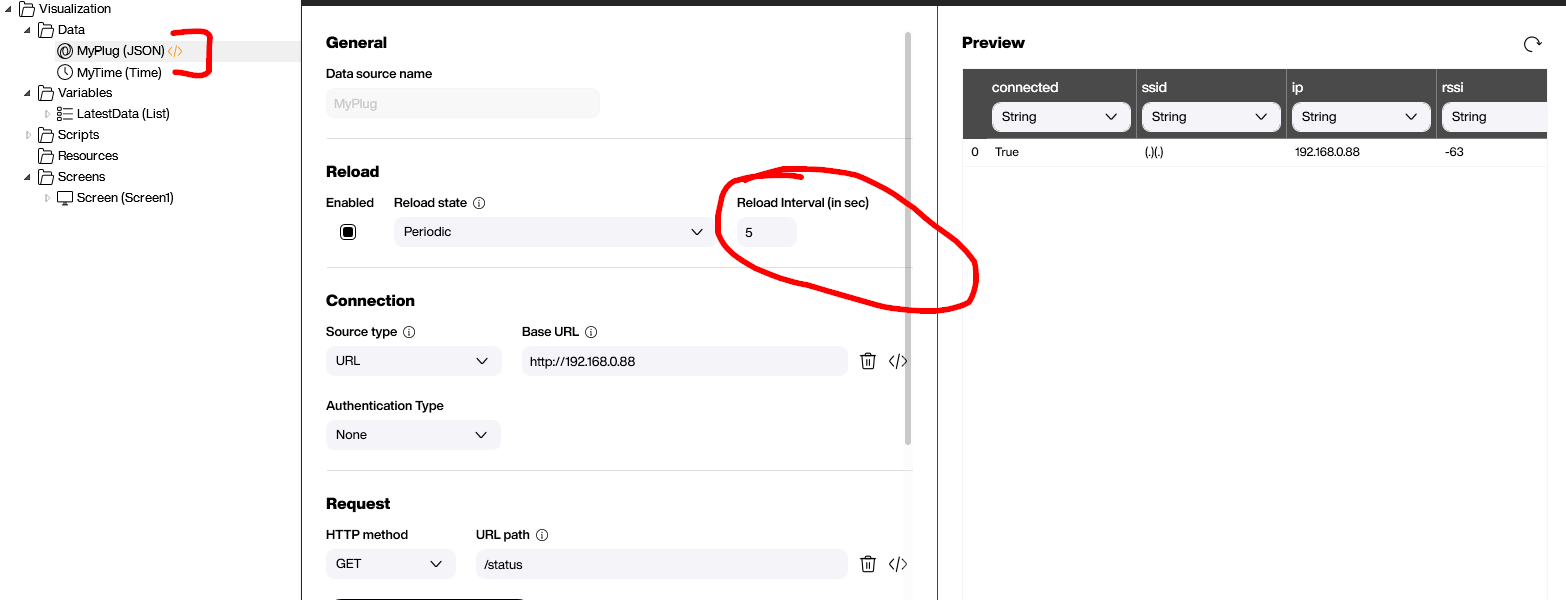
In Peakboard, the data source is a JSON call to the Shelly status API that is runs every 5 seconds. Please check the old article mentioned above for details. We set the Reload Interval to 5 seconds.
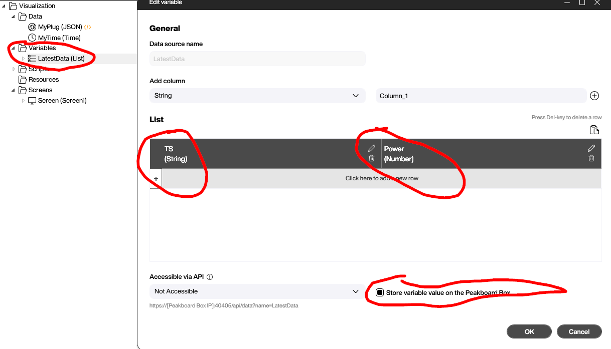
For the visualization, we store the data in a local table. To be more precise, we use a table-like variable.
The table only has two columns: TS (String) is the time stamp, and Power (Number) is the current power value. We also tick the Store variable value on the Peakboard box setting. That way, when the box is restarted, the previous data will still be there, and isn’t lost.
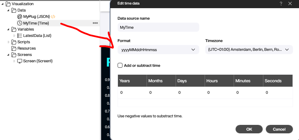
The next thing we need to add is a standard time source. That way, the current time will be available to us when we process a data point later.
Here’s the most important part: the Refreshed script of our JSON data source. It consists of two major steps:
- Add the latest data point to our local table. We do this by using the power element of the JSON output, as well as the timestamp provided by the time source.
- Check the number of elements in the table. If the number exceeds 1000, the first element (which is the oldest) will be deleted.
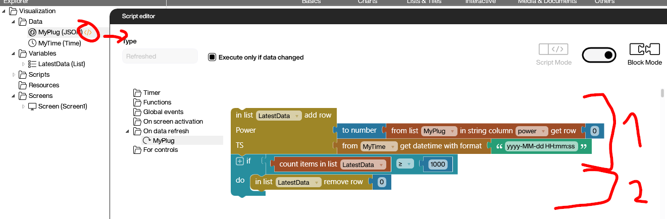
With this kind of pattern, the local table will always have the last 1000 data points. With a refresh rate of 5 seconds, the table will hold 1000 x 5 = 5000 sec = roughly 1,5 hours of data. So we can visualize what happened in he last 1,5 hours.
Visualizing the data
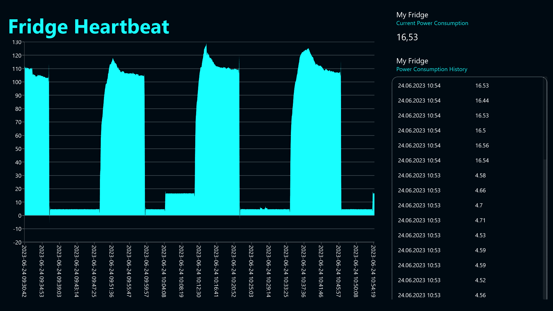
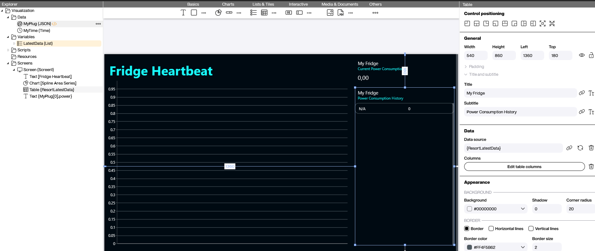
To visualize the data, we use a regular area chart. We put the power consumption on the y-axis. On the right side, we add a small table of the last 20 data points and a tile with the current value. Feel free to download the pbmx to find out more details.
The result
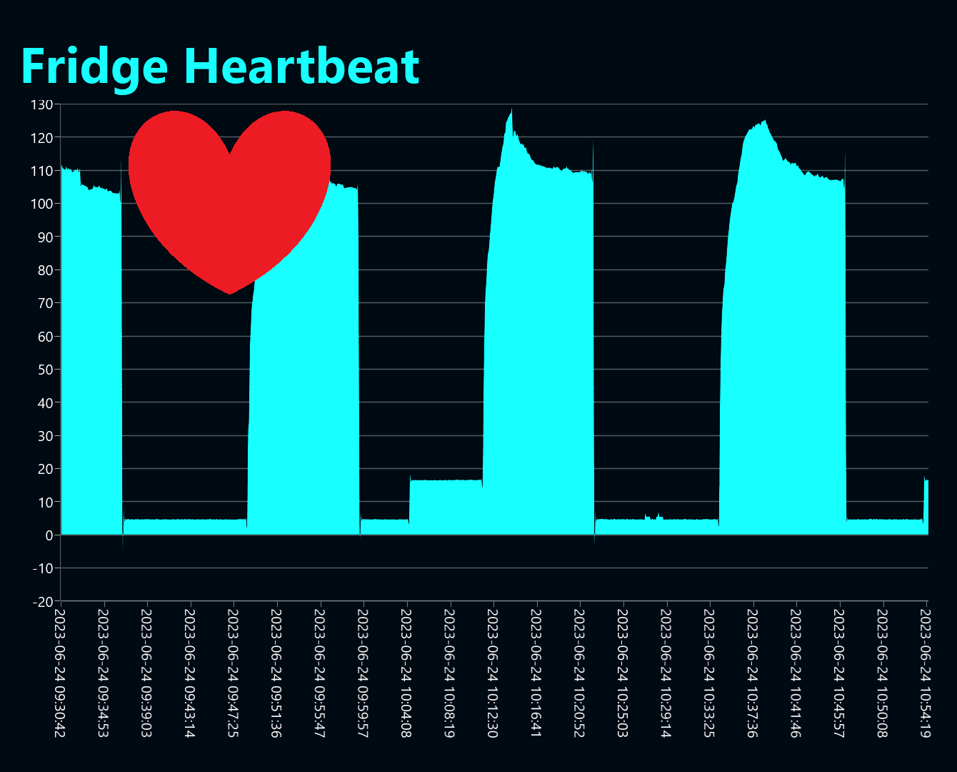
Here, you can see what our dashboard looks like, with a typical LG fridge with two doors. We can clearly see the periods of cooling (with high power consumption) and the periods when the fridge is idle (with low power consumption).
We can also see that the power consumption varies within a cooling period, which is probably related to the fridge’s internal processes. Initially, more power is needed to get the compressor to an efficient working state.
At the end of the cooling periods, we can also see that the power consumption goes up for a couple of seconds, in a needle-like peak, before it drops down into idle. Can anyone explain this?