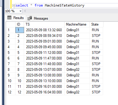
In this article, we learned how to store historical events in a SQL Server database. Every time a state changes, a new row is created with the timestamp and the name of the new state. As you can see in the sample data, there are two drilling machines switching between RUN and STOP throughout a regular working day.
The way the information is stored is of course unsuitable for end users and relatively hard to use for analysis. In this article, we will learn a best practice for how to handle this kind of data easily, by using intelligent SQL commands.
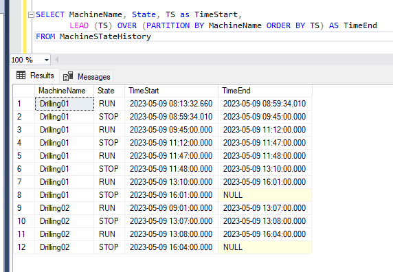
First, we want to transform the original data into a table where each state has a start time and an end time. That way, it’s much easier to do calculations. To achieve this, we use the SQL command LEAD. If you’ve never heard of it, please check out the documentation provided my Microsoft.
The LEAD command (shown below) says, “For each row, find the next row with a newer timestamp (order by TS)—but not just any next row—but the next state row of the same machine.” That’s where the PARTITION BY MachineName comes into play.
SELECT MachineName, State, TS as TimeStart,
	LEAD (TS) OVER (PARTITION BY MachineName ORDER BY TS) AS TimeEnd
FROM MachineStateHistory
This is what the resultset looks like:
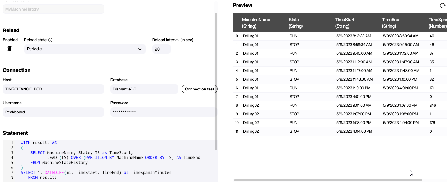
Later on, we will probably need the time difference between the start time and end time of each state, preferably in minutes. It wouldn’t be difficult to calculate this in Peakboard, but it’s a bit more elegant to let the SQL server do all the work by using the DataDiff command. Don’t forget to check the official documentation if you’re unfamiliar with the command.
There are several ways to combine DataDiff with the LEAD command. The easiest way is to wrap the LEAD statement in a WITH statement and then build a second SELECT around that resultset.
WITH results AS
(
	SELECT MachineName, State, TS as TimeStart,
		   LEAD (TS) OVER (PARTITION BY MachineName ORDER BY TS)
                AS TimeEnd
	FROM MachineStateHistory
)
SELECT *, DATEDIFF(mi, TimeStart, TimeEnd) as TimeSpanInMinutes
   FROM results;
And here’s what the resultset looks like in Peakboard Designer:
With that resultset, it’s super easy to calculate all related values by using a dataflow. This example shows how to aggregate the sum of all time span values and group it by machine and state. Then, it filters out anything that doesn’t have the state RUN. Then, it filters out anything that isn’t the machine Drilling01. And we end up with one single row representing the time that the Drilling01 machine has run in total.
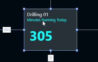
From there, it’s easy to finally bring it home. The aggregated number is just displayed in a simple tile. Mission accomplished.
Please keep one important lesson in mind: Although Peakboard offers multiple ways of manipulating data, it’s usually a wise choice to prepare the data for future use when creating the SQL statement. This can save lots of time later on and makes the whole data logic much easier to understand and maintain.